Load Profiles and Load Distribution
Information
- In PLANTA project there are three types of load distribution:
- Distribution with percentage load profiles (3/3, 5025, 5075, GSS, S, E)
- Distribution with load profiles which are based on a particular calculation method (CAP, BLD)
- Distribution with time grid load profiles (WEEK, YEAR, QUARTER, MONTH)
- Distribution with the manual load profile MAN load profile
- Distribution with manual time grid load profiles (PM_*)
- Linear distribution if no load profile has been selected
Details
- The Load profile parameter on a task resource in the Schedule module determines which load profile is applied to the respective task resource.
- Here, the required load profile can be selected via the listbox. If no load profile is selected, the resource will be distributed linearly.
- When you assign a resource to a task, the Default load profile of the resource is automatically adopted from the master data but can be changed on the resource assignment if necessary.
- The default load profile is determined per resource in the Default load profile field in the Resource Data Sheet.
- If the duration of a task resource deviates from the task duration (e.g. when several resources work on a task at different times), the effort is distributed over the duration of the task resource. The task duration only sets the time frame within which distribution takes place.
Notes
- Several load profiles are already included in the scope of supply of the PLANTA software. The creation of individual load profiles is currently not supported.
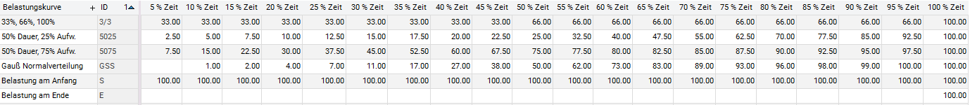
Distribution with Percentage Load Profiles
Information
- Load profiles for distribution on a percentage basis are defined in steps of 5%. The task runtime is divided into 20 intervals. During calculation of the loads, the Remaining duration of the task is divided by 20, and for each of the intervals thus generated, the Remaining effort is multiplied by the difference of the load percentage rates. This is how the load distribution is established.
- The general rule is: Duration and effort are set, the load is calculated.
Note
- Due to their division by 20, it may occur that the load will be distributed over more than one day when using the E and S load profiles. If the Remaining duration of the task is 60, then 60 / 20 = 3 load records are generated. See the examples under "Load at the end / start".
Example of utilization diagrams:
- 3/3
- 5025
- 5075
- GSS
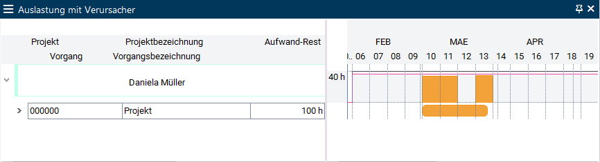
Taking into account of actual data in load profiles on a paercentage basis
- If the sum of the actual resource load deviates from the planned loads, scheduling readjusts the remaining loads to the load profile.
Example
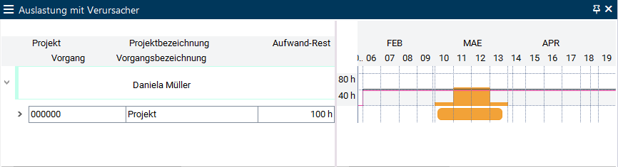
- Initial situation without time recording
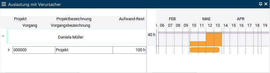
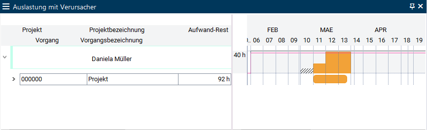
- Fewer Actual effort is recorded than initially planned. The total difference is additionally loaded on the first day after the date of time recording
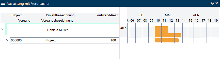
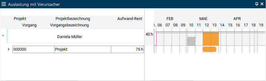
- More Actual effort is recorded than initially planned. Loading will not take place until the initial profile is reached again.
Load at the End / at the Start
Information
- If you use load profile E, loading takes place at the task end equivalent to load profile S.
- Due to the effective principle of distribution calculation, i.e. the division by 20, it may occur that the load will be distributed over more than one day when using the E and S load profiles. One load record is created per 20 days of task duration.
- In the following examples, E is used for demonstration purposes.
Examples
- Example 1: Resource R1 is planned for task A with a duration of 10 days and an effort of 100 h.
- Scheduling creates a load record with 100 h at the end of the task (on the last working day of the specified duration).
- Example 2: Resource R1 is planned for task B with a duration of 21 days and an effort of 100 h.
- Scheduling creates two load records at the end of the task (on the two last working days of the specified duration):
- Load record 1: 4.76 h
- Load record 2: 95,24h
- Scheduling creates two load records at the end of the task (on the two last working days of the specified duration):
Calculation for task C with Remaining duration = 21 days
- 21 / 20 = 1,05
- 2 load records are created: a load record which corresponds to the entire 20 days and one load record which corresponds to one day.
- The daily load amounts to: 4.76 (=100 / 21)
- The load is distributed in the following sequence according to the time interval steps.
- Load record 1: 4,76 x 1 = 4,76
- Load record 2: 4,76 x 20 = 95,24
- Example 3: Resource R1 is planned for task C with a duration of 44 days and an effort of 100 h.
- Scheduling creates three load records at the end of the task (on the three last working days of the specified duration).
- Load record 1: 9.09 h
- Load record 2: 45.45 h
- Load record 3: 45.45 h
- Scheduling creates three load records at the end of the task (on the three last working days of the specified duration).
Calculation for task C with Remaining duration = 44 days
- 44 / 20 = 2,2
- 3 load records will be created: 2 load records which correspond to the total of 2 x 20 days and a load record which corresponds to 4 days.
- The daily load amounts to: 2,27 (=100 / 44)
- The load is distributed in the following sequence according to the time interval steps.
- Load record 1: 2,27 x 4 = 9,09
- Load record 2: 2,27 x 20 = 45,45
- Load record 3: 2,27 x 20 = 45,45
Note
- The distribution sequence of the load under load profile S and with the existence of several load records is the exact reverse: large ones first and then the lower ones.
Gauss Load Profile (GSS)
Information
- When you use the Gauss load profile, the calculated start date of the resource does not correspond to the calculated start date of the task.
- Explanation: Across the task period, 20 intervals are created with ascending or descending values. Their first and last interval generate a distribution of effort and costs of 0 in the first and last 5% of the period. Only then will the effort or costs be planned with a profile with ascending and later descending values. Since records with 0 costs or effort are not written, the calculated start date of the resource is set to the date of the first record with positive effort or costs. On the task, the calculated start is set to today regardless.
- For tasks which have already started (with actual start), the effort or cost distribution is recalculated each time in accordance with the Gauss distribution, i.e.: the first interval is always 0. However, the effort or costs which have already incurred are offset as if the profile had been completely processed and the further calculation is based on a sum which equates to the sum from the initial calculation at the same point in time. If the incurred sum is higher than initially prescribed by the profile for the period from actual start to today, the calculated start of the resource is moved into the future. If the incurred sum is smaller, the calculated start is moved further towards the beginning.
Notes on operating with the GSS load profile:
- After initial scheduling (without actual loads), you can post exactly those sums on exactly those days that are prescribed by the profile. This ensures that the profile is processed exactly as initially planned.
- You can trigger an initial scheduling and freeze it as a baseline in a status report. You can then see the deviations in the status reports which will incur over time.
- or you can set a requested date for the task to prevent the profile from changing the end date. As soon as an actual start has been set, the profile will become steeper as the task progresses.
Distribution with Special Load Profiles
Information
- CAP, BLD load profiles are based on a special calculation method.
- CAP: the load in each period relative to available capacity. The effort of the assigned resource is dominant. In case of scheduling with adherence to float or capacity, the available capacity of the period is scheduled. The duration is calculated.
- BLD: Basic Load. It is used to plan the basic load projects along with the Max. load/day parameter. Without Max. load/day it takes effect as a linear load profile.
CAP Load Profile
Objectives
- Optimization of the capacity planning
- Calculation of the loads per day
- Calculation of the durations when loading in
Information
- The CAP load curve stands for capacity-oriented utilization.
- PLANTA project can calculate the loads per day and the task duration when effort is distributed. This takes into account how much remaining capacity of the resource is still available.
- This provides a solution for the following problem:
- The effort of a process is known and the duration of the process should be calculated. Existing loads of already loaded processes (also from other projects) and the available capacity of the resource are to be taken into account.
- The loads per day are to be effected in line with availabilities. This can also lead to processes being interrupted by more important processes or to processes being shortened if there is sufficient free capacity.
Note
- Planning with CAP is only effective if the Adjustment by effort parameter is activated for the resource. Otherwise, CP will ignore the CAP entry.
Planning with Adherence to Schedule with CAP
Information
- Planning with adherence to schedule by specifying the TA Remaining duration or the Max. load/day with optimized loading.
Details
- If no Remaining duration of the task is set, it is calculated based on
- Max. load/day of the resource assignment set: Remaining duration of the task = Remaining effort of the resource assignment / Max. load/day
- If no Max. load/day is set for the resource assignment either, the Remaining duration of the task is 1 day. The entire effort is planned on a day with overload.
- Max. load/day of the resource assignment set: Remaining duration of the task = Remaining effort of the resource assignment / Max. load/day
- The disposable capacity is planned for each day, if it is not restricted by a Max. load/day or Min. load/day . The loads on the individual days can vary.
- If no Max. load/day is set and the entire effort can be completely planned within the available capacity, the Remaining duration of the task may be reduced. This can result in very high daily loads.
- If it is not possible to plan in the total effort within the disposable capacity, the overload is distributed equally across all load records to days on which the resource is working.
Notes
- Even in planning with adherence to schedule, the resource-capacity will be optimized within the Remaining duration of the task. Practical experience has shown that overloads can be significantly reduced simply by setting CAPs while planning with adherence to schedule. This positive effect particularly occurs in employee-based planning.
- When planning with adherence to schedule with CAP , overloads are distributed equally across the resource’s working days to all load records.
Planning with Adherence to Total Float with CAP
Information
- Planning with adherence to total float by specifying the Remaining duration of the task or the Max. load/day of the resource assignment with optimized loading.
Details
- The Remaining duration of the task is calculated just as in planning with adherence to schedule but it may be extended up to the end of the total float time or of the planning horizon if there is insufficient capacity.
- The Calc. start is moved to the first day with remaining capacity, provided that its start is even earlier than the Latest start. Otherwise Calc. start = Latest start applies
- When planning with adherence to total float with CAP, overloads are distributed equally across the resource’s working day to all load records.
Planning with Adherence to Capacity with CAP
Information
- Planning with adherence to capacity by specifying the Remaining duration of the task or the Max. load/day of the resource assignment with optimized loading.
- TA Remaining duration is calculated in the same way as in the case of planning with adherence to schedule, but it can be extended due to a lack of capacity until the entire effort can be scheduled or until the end period of the resource calendar is reached. The PR Requested ED can be overrun.
- The TA Calc. start is moved to the first day with freely available capacity, provided that its start is yet earlier than the end date of the resource calendar . Otherwise, TA Calc. SD = end date of the resource calendar applies.
CAP with multiple resource assignments to the task
Information
- The resources are loaded independent of one another, and calculated durations and dates are summarized to the task.
Notes
- If the resources assigned to a task include some with CAP and some without, then the CAP resource assignments take precedence, i.e. the TA duration is determined from the CAP resource assignments. The non-CAP resource assignments are planned on the basis of the calculated TA duration and no resource capacity adjustment will be carried out for them.
- Exceptions:
- Remaining effort = 0 (CAP will not be taken into account in the calculation of the task duration)
- MAN load profile (cf. the corresponding chapter).
- Exceptions:
BLD (Basic Load) Load Profile
Information
- The Basic load (BLD) load profile can be used to distribute loads evenly across the entire float time of a task. In doing this,
- the daily load can be specified (via Max. load/day) or
- the daily load can be calculated from the Remaining effort of the task.
- This load profile is used for resource employment planning for accompanying activities. E.g.
- basic load tasks (e.g. 1h/day for service activities) or basic load projects
- project management (e.g. 1 hour/day throughout the entire duration of the project, or 100 hours distributed across the entire project duration)
Particularities of the BLD load profile
- If the Remaining duration of the task is specified, it will be taken into account.
- If the BLD load profile is assigned to a task and no Remaining duration is specified, the Remaining duration of the task will be calculated from Earliest start (= Calc. start) up to the Latest end (= Calc. end).
- If a value has been entered in Max. load/day , the Remaining effort = Max. load/day x Remaining duration will be calculated.
- If no value has been entered in the Max. load/day field, the Remaining effort will be distributed evenly over the Remaining duration ( behavior as in planning without load profile: linear load distribution).
- Tasks with a BLD resource assignment will always be planned with adherence to the schedule. I.e. no capacity adjustement is carried out for them.
- Resources are not scheduled for the time of their vacation.
- The task can be stretched across the complete project duration if the Hammock task parameter has been activated (e.g. for project management or basic load projects).
- A hammock task can be stretched across certain project tasks by using links. For example, the link predecessor can be the project kick-off milestone and the successor can be the Project end milestone. The hammock task will be stretched between these two tasks if it is connected to both tasks by links.
Distribution with Time Grid Load Profiles: WEEK, MONTH, QUARTER, YEAR
Information
- If you use the WEEK, MONTH, QUARTER or YEAR load profiles, only one load record is created per week, month, quarter, or year.
- The objective of the use of these load profiles is an acceleration of long-term analysis (e.g. utilization diagrams) by the reduction of load records.
Notes
- When you use the WEEK, MONTH, QUARTER, and YEAR load profiles,
- Remaining duration or requested dates (Requested start and Requested end) of the task and Remaining effort of the task resource(s) must be specified.
- the Max. load/day parameter has no effect.
Details on remaining load
Information
- In the first step, scheduling calculates the load records exactly to the day (in the background).
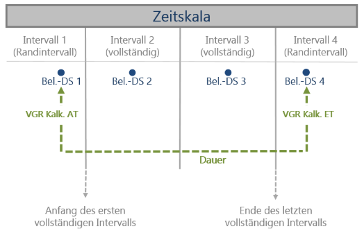
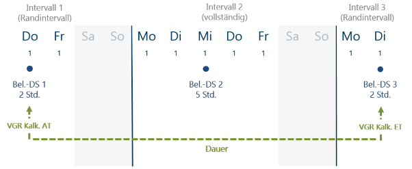
- In the next step, scheduling summarizes the load records to the following points in time:
- for complete intervals to the middle of the respective interval
- WEEK: Loading only on each Wednesday of a week
- MONTH: Loading only on the 15th day of a month
- QUARTER : Loading only on the 15th day of each central month of a quarter
- YEAR: Loading only on July 15th of a year
- Please note that scheduling does not treat the 15th of a month as a real date but only as an interval marker. I.e., if the 15th is a non-working day, loading takes place on that day anyway.
- for the margin intervals it is loaded on the Calc. start of the resource assignment and Calc. end) of the resource assignment. This means:
- The date of the first planned load record equates to the Calc. start of the resource assignment.
- The date of the last planned load record equates to the Calc. end) of the resource assignment.
- for complete intervals to the middle of the respective interval
Schematic display
Examples of application
- A task with a duration of 9 days and a resource assignment with WEEK load profile and Remaining effort = 9 h begins on a Thursday and ends a week later on a Tuesday.
- In the first step, scheduling distributes the 9 hours evenly among the 9 days, resulting in a load of 1 hour per working day.
- In the second step, scheduling summarizes the distributed hours to one load record per interval.
- The 1st summarized load record contains the data from Thu – Fri and has TAR Calc. start (=Thursday of the first week) as a date.
- The 2nd summarized load record contains the data from Mon – Fri and has the Wednesday of the second week as a date
- The 3rd summarized load record contains the data from Monday – Tuesday and has TAR Calc. end (= Tuesday of the 3rd week).
- As a result of summarization, inaccuracies may occur in the summarized values. Cyclical replanning is recommended.
- The grid for the analyses (e.g. for utilization diagram) should be equal to, or greater than the summarization time grid; e.g. if the display is shown to the day for a summary on an annual time grid, all loads would appear on 07/15.
Details on actual loads
Information
- Since the recording of hours worked is is carried out per day, the actual records exist day-wise, independent of the selected grid.
Distribution with MAN Load Profile
Information
- Load records of MAN resources have an effect similar to that of an actual date. The planning data is frozen and is not moved by the scheduling.
- Actual dates do not change the MAN planning either.
- The MAN load profile is set manually on the resource assignment.
- Effort is entered in the Remaining effort field in the load record.
- The old value in the Remaining load of the load record is retained and can be changed manually.
- Remaining effort on the resource assignment = sum of the Remaining load of all corresponding load records, i.e. the loads will be cumulated upwards.
Typical application in practice
- Free capacity load distribution across the task duration.
- Manual distribution of loads to achieve capacity adjustment.
- Project meetings on fixed dates
Particularities of the MAN load profile
- The Active today’s line does not move dates planned with MAN
- Links: They take effect until they encounter MAN dates. (e.g. when resources are loaded multiple times with MAN and CAP)
- The impact of setting a resource with MAN and other resources with other load profiles on a hammock task, summary task, or BLDare similar to that in the example cited above:
- The dates of the MAN planned resources will not be moved.
- The impact of setting a resource with MAN and other resources with other load profiles on a hammock task, summary task, or BLDare similar to that in the example cited above:
- Hammock task duration or summary task ≥ MAN period
- earliest start ≤ first MAN date
- latest end ≥ latest MAN date
- In the case of several resources with MAN, the earliest and latest dates of all MAN resources are used to plan the TA.
- Via TA Requested start , the task can only start earlier than the earliest MAN planning.
- As a result of TA Requested end , the task can only start earlier than the latest MAN planning.
- Split parameter = : The parameter has no influence on of MAN resources. For resources which are not planned with MAN, this parameter has the same effect as before.
- Load records of MAN resources can only be deleted manually.
- Planning hours of the MAN load profile that are earlier in time than the first work reporting are deleted and not distributed to future loadings.
- Reporting of hours worked with a different value than planned do not affect the other load records.
- The recording of hours worked does not change the planned hours.
- Hours planned for task resources using MAN load profile are not shifted in scheduling.
Distribution with Manual Time Grid Load Profiles PM_* (persistant manual)
Load profiles for manual distribution of effort in time intervals
- PM_DAY
- PM_MONTH
- PM_WEEK
- PM_QUART
- PM_YEAR
They function in a way similar to normal time grid load profiles, with the difference that the distribution can either be carried out manually immediately (manual) or can be adjusted manually after initial automatic distribution. The manually generated or changed records are no longer changed by the scheduling (persistent).
Examples of application: In contrast to normal load profiles with time grid, manual load profiles with time grid allows. e.g., to interrupt the planning of a resource for a task.
Procedure
- When using the PM_grid load profiles, you can choose between two procedures.
- Procedure 1
- Define effort and requested dates on the resource assignment (for this purpose, see the note further below) and calculate the schedule. This effort is automatically distributed according to the equivalent time grid load profile (PM_WEEK according to WEEK, PM_MONTH according to MONTH, PM_QUART according to QUARTER and PM_YEAR according to YEAR), but only initially. Load data can then be edited manually; the load data records remain unchanged for any subsequent calculation. Only the remaining load is recalculated (e.g., in contrast to MAN load profile, actual load is subtracted from the remaining load) and summarized to the resource assignments.
- This procedure can e.g. be used as an input assistance.
- Procedure 2
- Initially you manually create load records in accordance with the selected interval. With this procedure, the manually created records are no longer changed from the first calculation on. The data is simply summarized upwards. In any subsequent calculation, the load records also remain unchanged. Only the remaining load is recalculated (e.g., in contrast to MAN load profile, actual load is subtracted from the remaining load) and summarized to the resource assignments.
- This procedure is recommended by PLANTA.
- Procedure 1
Notes
- For a task that possesses a resource assignment with PM_interval load profile, the following parameters are set automatically
Caution
- Due to these limitations and in order to guarantee the correct functionality of the PM_grid load profile you are advised to use requested dates instead of remaining duration in both cases mentioned above.
Particularities of Manual Load Profiles with Time Grid
Notes
- The general information and details for the intervals and the distribution of load records per interval which are described in the "Load Profiles with Time Grid: WEEK, MONTH, QUARTER, YEAR" section, also apply to manual time grid load profiles
- In the following, only particularities of the manual time grid load profiles are described.
Details
- Since only one Remaining record (plan record) is allowed per interval, every further remaining record created in the same interval is consolidated with the record which was created first, i.e. the load is added to that of the first record.
Details on Remaining and Actual Effort
- For PM_Grid load profiles you have the option to control the planned effort which remains after reporting of hpurs worked (actual effort) in a different way:
- Variant 1: Automated correction of the remaining effort in underpostings/overpostings to better adjust the planning to the actual situation and utilize the remaining effort more efficiently. Unused effort from previous periods is made available to future periods and, conversely, if more effort was posted than planned, the effort is subtracted from future periods. For further information on this, please see Effort Adjustment for PM_Grid Load Profiles.
- Variant 2: No automated correction. Here, the remaining effort behaves as follows:
- If the entire planned effort is reported to an interval as actual effort, the remaining effort is set to 0, the respective remaining record (planning record), however, is retained.
- If more hours worked are reported in an interval than planned, the remaining effort is set to 0 as well, but the total effort is increased as those hours are not subtracted from the planned effort of other intervals.
- If hours are reported in an unplanned interval, the total effort is increased since the hours cannot be subtracted from the effort planned in other intervals.
before work reporting
after work reporting

Caution
When planning with PM_Grid load profiles > PM_DAY, there may be differences in overloads in DT472 Load and DT468 Period to be considered. If there are, e.g., overloads at period level, they may be compensated in the week or month planning data and may therefore not be specified in DT472.
Reason: The effort is linearized to grid granularity, as the storage only contains the total effort, etc. over the respective period and the number of working days affected. Overloads are thus only indicated on grid granularity. Overload only arises in a load record when the remaining effort exceeds the availability in the entire period in question.
Differences Between MAN and PM_DAY
| load profile | PM_DAY | |
|---|---|---|
| There is only one record per day (period): remaining or actual. If actual hours are recorded for the day, the entire remainder for the day in question is deleted during schedule calculation. | ≠ | There is one remaining record and possibly several actual records per day (period). The remaining record is always retained, the actual records are always added. |
| The recording of hours worked does not change the planned hours. | ≠ | The reported hours are subtracted from the planned hours. If a new load record is added in a defined interval, the remaining effort is automatically increased accordingly. |
| Planning hours of the MAN load profile that are earlier in time than the first work reporting are deleted and not distributed to future loadings. | ≠ | Planning hours of the PM_DAY load profile that are earlier in time than the first work reporting are deleted and not distributed to future loadings. | |
| Reporting of hours worked with a different value than planned do not affect the other load records. | = | Reporting of hours worked with a different value than planned do not affect the other load records. |
| Scheduling does not shift hours planned of task resources which use the MAN load profile. | = | Scheduling does not shift hours planned of task resources which use the PM_DAY load profile. |
No Load Profile: Linear Load Distribution
Information
- In linear load distribution the Remaining effort of the task resource is distributed linearly over the duration (duration of the task resource or of the task).
- Overloads are not adjusted but only identified.
- The linear load distribution is carried out if no load profile has been selected for a task resource.
Example
- Remaining duration = 10 days
- Remaining effort = 100 hours
- Hence, load 100/10=10 hours per day
- If the resource has an availability of 8 hours per day, 2 hours of overload are shown on each day.
-
Page:Scheduling (Calculation of the Projects) (PLANTA project/portfolio)